When a Wrong Model Agrees With Itself

TL;DR: The last note let a wrong model choose what evidence to buy, then quietly gave it the true error model before inference. Removing that mercy changes the shape of the failure. The old “one bad column” widens into a low-$\hat\rho$ region where the same assumption first over-buys repeated cheap measurements and then over-trusts the agreement among them. At true $\rho=1$ and assumed $\hat\rho=0.05$, misspecifying allocation alone loses nothing, and misspecifying inference alone loses nothing, but coupling the two loses 21.2 points of recall. Even before screening, the model’s mean-squared error is 7.15 times the posterior variance it claims; inside the shortlist that ratio rises to 12.6 times. It buys precise evidence and then suppresses it.

The last note ended by naming the simplification it had been built around. I let an assumed $\hat\rho$ decide how the budget should be split, generated the measurements under the true $\rho$, and then interpreted those measurements using the true $\rho$ again. The model was allowed to make one mistake and then an oracle corrected it before that mistake reached the ranking.

That was the right experiment for isolating the price of a wrong allocation. It is not how a real decision system gets to be wrong.

If I do not know $\rho$ when deciding what to measure, I do not suddenly know it after the measurements arrive. The same belief that sets the acquisition policy will usually set the posterior weights too. This note removes the correction and asks what happens when a wrong model is allowed to remain internally consistent from purchase to interpretation.

The answer is not merely that two mistakes are worse than one. The interesting case is where neither mistake looks costly on its own, but their composition is.

The Missing Second Mistake

The machinery is unchanged from “The Price of a Wrong Prior”. There are $N=4000$ compounds with hidden qualities

\[q_i \sim \mathcal{N}(0,1),\]

and the top $H=80$ are the genuine hits. One free cheap measurement screens the full population; the top $M=500$ enter a shortlist. A budget of $B=16{,}000$, or 32 units per shortlisted compound, is then spent uniformly. The cheap instrument has $\sigma_c=1.0$ and costs one unit. The precise instrument has $\sigma_e=0.35$ and costs $r=32$. After the follow-up measurements, the top $L=100$ posterior means are selected and recall of the true 80 is measured.

Repeated measurements from instrument $j$ contain a shared component and a fresh component:

\[y_{ijk}=q_i+\sqrt{\rho}\,\sigma_j z_{ij} +\sqrt{1-\rho}\,\sigma_j\eta_{ijk}.\]

Averaging $K$ reads therefore gives an effective error variance

\[v_j(K;\rho)=\sigma_j^2\left(\rho+\frac{1-\rho}{K}\right).\]

The private term shrinks with $K$; the shared term does not. The allocator uses $\hat\rho$ to choose the cheap/precise split that maximises assumed posterior precision. The inference model then turns the purchased means into

\[\hat\mu_i= \frac{\hat\tau_c\bar y_{ci}+\hat\tau_e\bar y_{ei}} {1+\hat\tau_c+\hat\tau_e}, \qquad \hat\tau_j=\frac{1}{v_j(K_j;\hat\rho)}.\]

The new part is a four-way decomposition, all evaluated on paired random draws:

1. oracle: true $\rho$ for allocation and inference;
2. wrong allocation only: $\hat\rho$ for allocation, true $\rho$ for inference;
3. wrong inference only: true $\rho$ for allocation, $\hat\rho$ for inference;
4. both wrong: $\hat\rho$ for both allocation and inference.

I ran 256 paired Monte Carlo replicates at each point on a grid of 21 true values of $\rho$ and 41 assumed values of $\hat\rho$. The bands below are the 16th to 84th percentiles.

One Bad Column Becomes a Bad Wedge

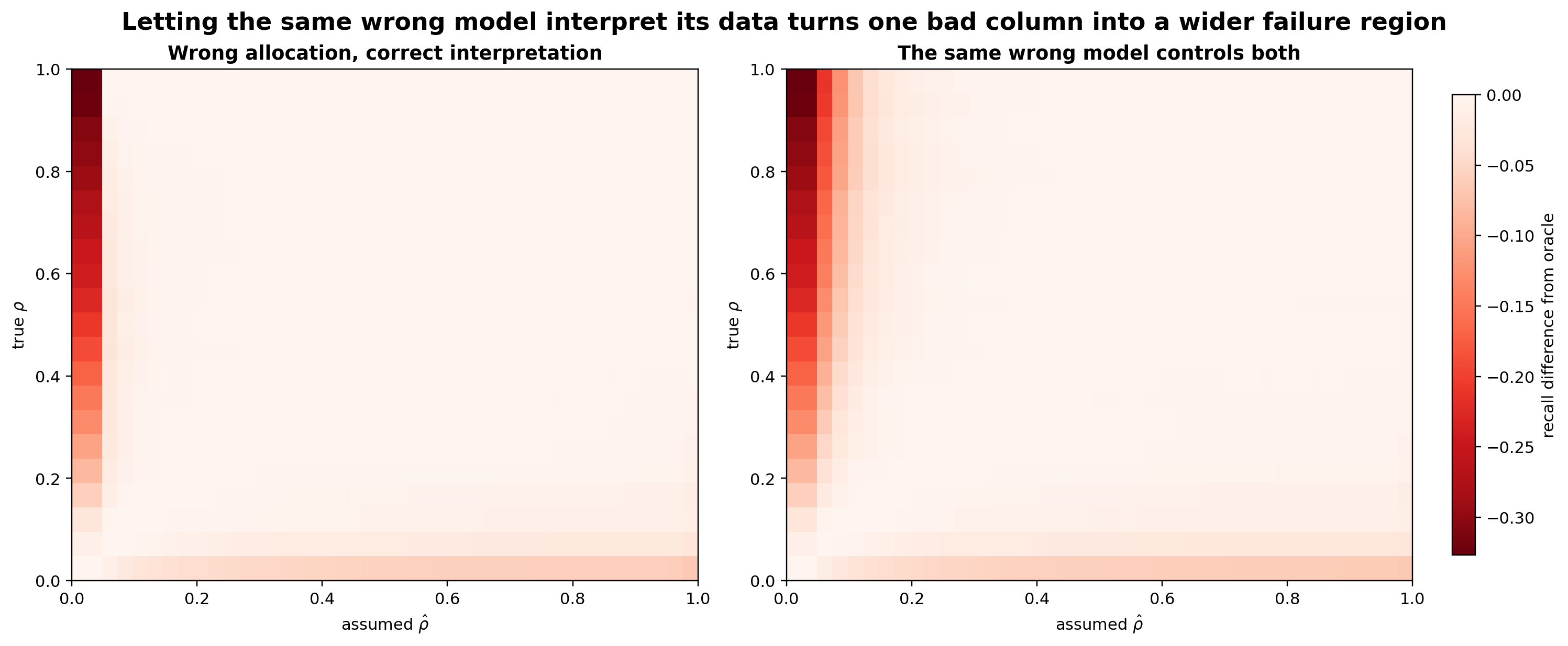
The left panel is the previous experiment at higher Monte Carlo resolution. It recovers the same shape: almost all of the damage is concentrated at $\hat\rho=0$. At true $\rho=1$, the oracle recall is $0.694$ and the confidently independent allocator falls to $0.367$, a loss of 32.7 points. Once $\hat\rho$ moves even slightly above zero, correct downstream interpretation repairs almost everything.

The right panel is what happens when that repair is removed. The worst point does not become much worse; at $\hat\rho=0$ the model buys only cheap measurements, and changing the posterior scale cannot change their rank order. What changes is the width of the failure. Small positive values of $\hat\rho$ are no longer safe.

At true $\rho=1$:

• $\hat\rho=0.05$ loses 21.2 points of recall;
• $\hat\rho=0.10$ still loses 6.8 points;
• $\hat\rho=0.20$ loses about 1.1 points.

In this grid, the joint system needs $\hat\rho\approx0.225$ before its mean recall comes within one point of the oracle at true $\rho=1$. At true $\rho=0.8$, the corresponding threshold is about $0.25$. The last note’s practical comfort — that almost any small hedge toward bias was enough — was a property of correcting the model before inference. It does not survive the closed loop.

Zero Plus Zero Is Not Zero

The cleanest point in the grid is true $\rho=1$, assumed $\hat\rho=0.05$:

allocation model	inference model	mean recall@100
true $\rho$	true $\rho$	0.694
wrong $\hat\rho$	true $\rho$	0.694
true $\rho$	wrong $\hat\rho$	0.694
wrong $\hat\rho$	wrong $\hat\rho$	0.482

Wrong allocation alone costs exactly zero in these paired runs. Wrong inference alone costs exactly zero. Put them together and 21.2 points disappear, with a paired 16th–84th percentile loss of $[-0.263,-0.163]$.

I measured that non-additivity directly as

\[I=(R_{11}-R_{00})-(R_{10}-R_{00})-(R_{01}-R_{00}) =R_{11}-R_{10}-R_{01}+R_{00},\]

where $R_{00}$ is the oracle, $R_{10}$ has only the allocation wrong, $R_{01}$ has only inference wrong, and $R_{11}$ has both wrong. Here $I=-0.212$: the entire loss is an interaction that neither isolated test can see.

The exact zeros at $\rho=1$ have a useful explanation. The oracle buys one precise read. With one read, $v_j(1;\rho)=\sigma_j^2$ regardless of $\rho$, so giving the oracle allocation a wrong inference value cannot change its weights. In the other isolated test, the $\hat\rho=0.05$ allocator buys both instruments; once those measurements are interpreted with the true $\rho=1$, repeated reads have no private noise left to average and the correct posterior collapses back to the same two instrument-level observations as the oracle.

Each isolated test is rescued by the half of the system that still knows the truth. The coupled system has no such rescue.

This is not only an endpoint trick. At true $\rho=0.8$ and $\hat\rho=0.05$, wrong allocation alone loses 1.7 points and wrong inference alone loses 0.4. Both together lose 17.9 points; 15.8 of those points are the interaction. The same structure remains after the exact cancellation is gone.

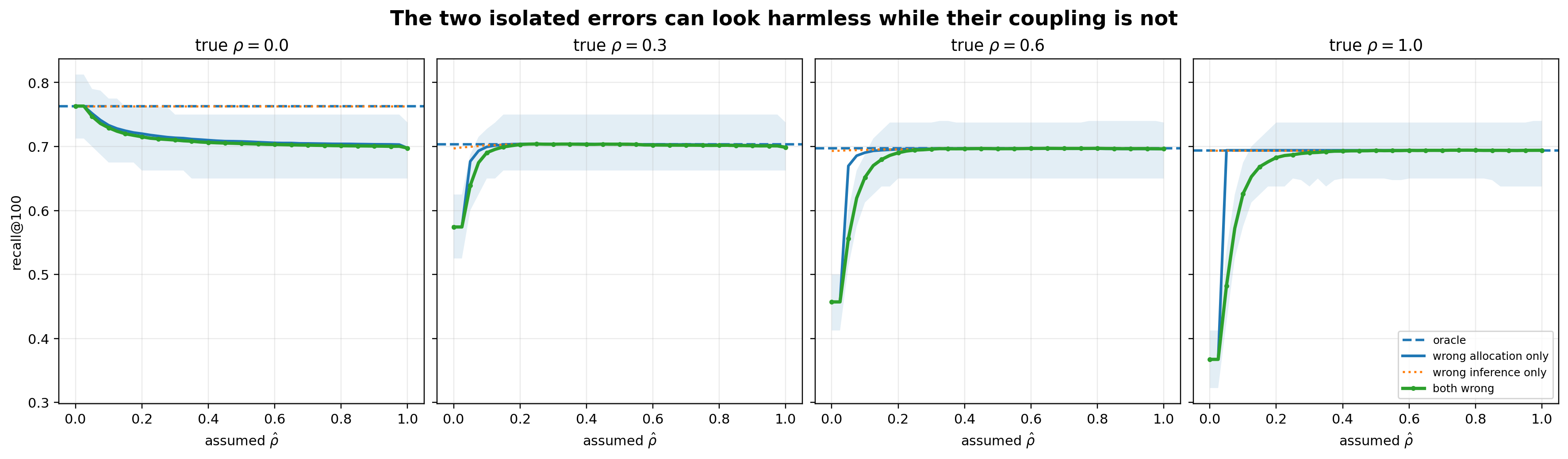
The line plot makes the coupling visible. The allocation-only curve climbs back onto the oracle almost immediately. The inference-only curve is also nearly flat. The joint curve recovers much more slowly because $\hat\rho$ appears twice: first in the evidence the system purchases, then in the meaning it assigns to that evidence.

It Buys Precision and Then Refuses to Believe It

At true $\rho=1$ and assumed $\hat\rho=0.05$, the optimiser buys 18.455 extra cheap reads, for 19.455 cheap reads including the free screen, plus 0.423 precise-read equivalents. The fractional count is the same continuous-effort abstraction used in the preceding note; I test integer reads below.

Under the true model, repeated cheap reads at $\rho=1$ do not average down at all. Their variance is still $1.0$. The precise instrument’s variance is $0.1225$. Correct inference on the purchased data therefore assigns posterior weight 0.098 to the cheap evidence and 0.803 to the precise evidence, with the remaining weight on the prior.

The wrong model reads the same purchase in almost the opposite way. It assigns weight 0.689 to the cheap evidence and only 0.242 to the precise evidence. It did pay for precision, but its belief in cheap-read independence turns the repeated cheap bias into apparent confirmation and pushes the actually informative measurement toward the edge of the posterior.

That is the self-confirming loop in one sentence:

Low $\hat\rho$ makes repeated cheap measurements look worth buying, and the fact that they were bought makes their agreement look worth trusting.

The acquisition policy creates exactly the evidence pattern its inference model is predisposed to overvalue.

Agreement Is Not Calibration

Internal consistency also makes the system more confident than its accuracy allows. Under the assumed model, the claimed posterior variance is

\[\hat V=\frac{1}{1+\hat\tau_c+\hat\tau_e}.\]

Because the weights were computed from the wrong variances, the actual mean-squared error is

\[\operatorname{MSE}(\hat\mu)= (w_c+w_e-1)^2+w_c^2v_c+w_e^2v_e,\]

with $v_c$ and $v_e$ evaluated under the true $\rho$.

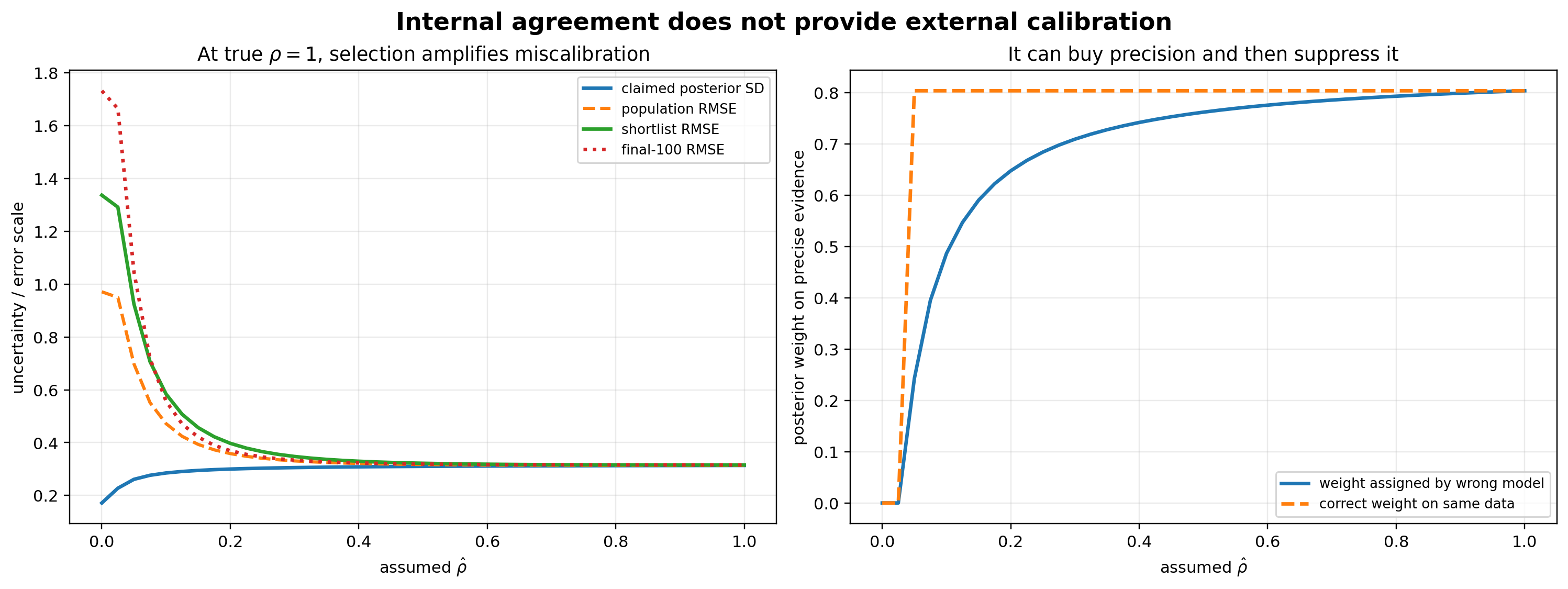
At true $\rho=1$ and $\hat\rho=0.05$, the model claims posterior variance $0.068$. Before any selection is imposed, its actual MSE under the original population model is $0.487$: 7.15 times larger. In standard-deviation terms, it reports $0.261$ while the population RMSE is $0.698$.

That calculation is deliberately analytic, but it averages over the original $q_i\sim\mathcal{N}(0,1)$ population. The ranking system does not act on a random compound. It acts after the cheap screen has selected compounds with unusually high observed scores, then acts again on the final 100. I therefore repeated the calibration calculation inside those two selected sets. The shortlist MSE rises to $0.856$, or 12.56 times the claimed variance. Among the final 100, it reaches $1.096$, or 16.08 times the claimed variance. Selection does not create the misspecification, but it concentrates the system exactly where that misspecification is most costly.

At $\hat\rho=0$, the population-level mismatch is already extreme. Thirty-three cheap reads produce a claimed variance of $0.029$, while population MSE is $0.943$, a 32-fold variance error. Inside the shortlist the ratio is 60.7-fold; among the final 100 it is about 102-fold. The model reports a posterior standard deviation of $0.171$ while the decisions it treats as most promising are the ones furthest outside that confidence claim.

This is the part that ranking recall alone does not expose. A wrong model can lose hits and know it is uncertain, or it can lose hits while becoming more certain. The second is the more dangerous failure because every internal diagnostic built from the same assumption can agree that the posterior is sharp.

The agreement is real. It is simply not independent evidence.

The Reverse Mistake Is Still Bounded

The asymmetry from the previous note remains. When true $\rho=0$ and assumed $\hat\rho=1$, the joint policy falls from $0.763$ recall to $0.698$, a loss of 6.6 points. In this corner the damage still comes from allocation: the model overpays for precise measurements when cheap independent reads could have averaged down efficiently. The wrong inference adds nothing because a single read from either instrument has the same marginal variance for every assumed $\rho$.

So the old directional lesson survives: confidently denying shared bias is more dangerous than confidently assuming it. What changes is how much hedging is enough. Once acquisition and inference share the same prior, $\hat\rho=0.1$ is no longer a nearly complete defence against true high correlation.

It Is Not a Fractional-Read Artifact

The main experiment permits fractional precise-read equivalents because the preceding price model treats budget as divisible effort. That abstraction could exaggerate the interaction by creating allocations such as 0.423 of a precise read, so I reran the critical region with integer-only purchases. I doubled the per-compound budget to 64 units, kept the precise-read price at 32, and restricted the optimiser to whole reads.

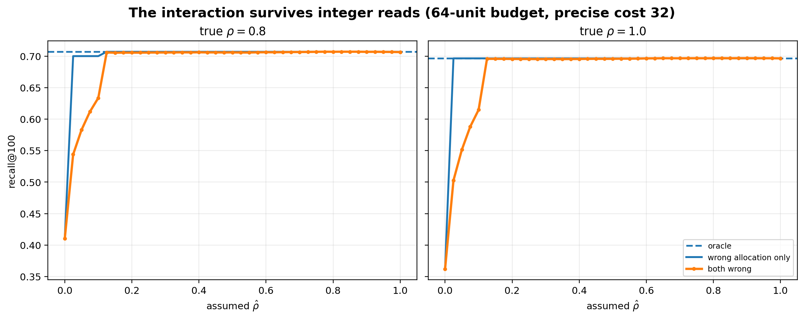
At true $\rho=1$ and $\hat\rho=0.05$, the wrong allocator buys 33 total cheap reads and one precise read. Correct interpretation of that allocation remains on the oracle at $0.697$ recall. Let the same wrong model interpret it and recall falls to $0.551$, a 14.5-point loss. At true $\rho=0.8$, the corresponding joint loss is 12.4 points, of which 11.6 are interaction.

The exact numbers move because the budget and feasible allocations changed. The coupling does not.

Where This Lands

1. Component-wise robustness is not closed-loop robustness. Testing a misspecified allocator with an oracle interpreter, then a misspecified interpreter with an oracle allocation, can let both components pass while their composition fails. Each isolated test conditions away the feedback path that makes the error self-reinforcing.

2. The same assumption can affect both the evidence collected and the authority granted to it. Low $\hat\rho$ first purchases repeated cheap measurements because their noise appears averageable. It then treats their repeated agreement as independent confirmation. Those are not two additive errors; they are one loop.

3. Internal agreement is not calibration. At the critical point, population MSE is seven times the variance the system reports; inside the shortlist it is more than twelve times. Every module can agree because every module inherited the same wrong covariance model. Agreement only becomes corroboration when the routes to agreement can fail independently.

4. A hedge must survive inference, not only acquisition. In the allocation-only experiment, $\hat\rho=0.1$ was enough to erase almost all risk. In the joint experiment it still loses 6.8 recall points at true $\rho=1$. Robust purchasing without robust weighting is only half a defence.

What This Is Not

Still a toy. The two instruments share one $\rho$ value; their $\sigma$ values and prices are known; the prior is correctly specified; every shortlisted compound receives the same allocation; and the observation model is Gaussian. The main run uses divisible measurement effort, although the integer experiment shows that the interaction does not depend on it. The exact 21.2-point loss is a property of this budget, this price, these instruments, and the $\rho=1$ endpoint — not a constant to carry into another system.

The part I would carry is the diagnostic structure. If one uncertain assumption controls both which evidence enters a system and how that evidence is weighted, perturbing each component in isolation is not enough. The joint path has to be tested, and calibration has to be checked against something that does not inherit the same assumption.

The next question is no longer how much a wrong $\rho$ costs. It is whether the system should spend part of its budget learning $\rho$ — through deliberate overlap, controls, or repeated cross-instrument measurements — while it is using those instruments to search.

A wrong model does not become safer because every module agrees with it. It becomes harder to contradict.