The Price of a Wrong Prior

TL;DR: Away from the crossing price, a wrong belief about the error correlation $\rho$ is mostly harmless — except for one corner. Confidently assuming errors are independent ($\hat\rho=0$) when they are not costs up to 33 points of recall; the reverse mistake ($\hat\rho=1$ when $\rho=0$) costs at most 6. Any hedge toward believing bias might exist — even $\hat\rho=0.1$ — erases almost all of the risk. The mechanism: a cheap instrument’s bias floor can coincide with total ignorance, a precise instrument’s cannot, so over-trusting the noisy one is unbounded and over-trusting the sharp one is not.

The last note ended with a confession pointed straight at itself: the price-aware split “prices precision correctly only because I told it the prices.” $\sigma_c$, $\sigma_e$, and $\rho$ were all handed to the optimizer as known constants. In the wild you do not know how correlated your instrument’s errors are — you assume a value, $\hat\rho$, and hope it is close enough. This note asks the obvious next question: what does a wrong $\hat\rho$ cost you?

The First Design Was a Dead End

The natural place to test this felt like the crossing itself — $r \approx 8$, the exact price where all-cheap and all-precise tied in the last note. I built the experiment there first: sweep an assumed $\hat\rho$ against a true $\rho$, watch the price-aware split’s allocation degrade.

It didn’t degrade. The heatmap came back almost perfectly flat, and worse, at the one point that looked like it mattered — $\hat\rho \to 1$ — the “effect” turned out to be a tie-breaking artifact in my own optimizer, not a real prediction. That was worth catching before writing anything about it, and it is worth explaining why it happened, because the reason is the actual finding of this section.

The crossing $r^*$ is, by definition, the price at which two very different strategies perform identically. That is a point of maximum indifference to your allocation — almost anything you buy there works about as well as anything else, so a wrong belief about $\rho$ has nothing costly to be wrong about. Testing misspecification at the point of maximum indifference was exactly backwards. The place a wrong prior can hurt you is where the correct allocation is a strong, decisive skew — where being wrong doesn’t just cost you a few percentage points at the margin, it puts you on the wrong side of the argument entirely.

There was a second, smaller thing to fix alongside this: at the original per-compound budget ($8$ units against a precise-read price of $r=32$), the whole budget could buy at most a quarter of a precise read’s worth of averaging ($8/32=0.25$) — too thin a margin to be worth diverting from cheap reads except when $\hat\rho$ was already large, so the optimizer’s choice collapsed to a hard corner (all-cheap or the full sliver of precise) for almost every belief. I raised the per-compound budget fourfold, to $32$ units — exactly one precise read’s worth — so the split has real interior room to trade a fraction of a precise read against cheap reads; everything else — $N$, $H$, $M$, $L$, $\sigma_c$, $\sigma_e$ — is unchanged from the last note.

The Setup

Same machinery as “The Price of Precision,” with two changes: a larger per-compound budget, and a fixed cost ratio moved off the crossing. Four thousand compounds, hidden qualities $q_i \sim \mathcal{N}(0,1)$, the genuine hits the top $H=80$. A free cheap screen scores all of them; the top $M=500$ form a shortlist. A budget of $B=16{,}000$ (32 units per shortlisted compound) is spent there. Cheap reads cost $1$ and have $\sigma_c=1.0$; precise reads cost $r=32$ and have $\sigma_e=0.35$ — the same instruments as before, at a price well past the crossing, where all-cheap should clearly beat all-precise if $\rho$ is small.

The allocation problem is unchanged in spirit: for an assumed $\hat\rho$, choose how many extra cheap reads and how many precise reads to buy with the per-compound budget, maximising assumed posterior precision. What’s new is that this choice is now made with $\hat\rho$, while the data is generated with a possibly different true $\rho$, and downstream interpretation of whatever reads get bought uses the true $\rho$ — the mistake under test is mispricing precision, not also misreading your own instruments afterwards. (See “What This Is Not” for why that split is the honest scope here.) Eighty replicates; bands are 16th–84th percentile.

The Heatmap Has One Bad Column

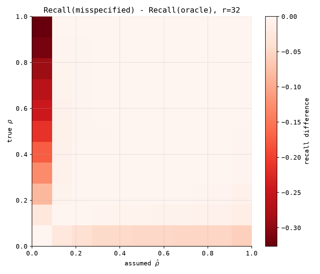
Sweep $\hat\rho$ against $\rho$ at $r=32$ and almost the entire grid is a pale, unremarkable near-zero. Then there is one column that is not: $\hat\rho = 0$. Believing with certainty that your instruments’ errors are independent, when they are not, costs recall that climbs steadily with how wrong you are — from nothing at $\rho=0$ to roughly 33 points of recall at $\rho=1$, a paired, statistically solid loss ($16$–$84$ band $[-0.38, -0.26]$, nowhere near zero). In absolute terms that is the oracle split’s $0.69$ recall at $\rho=1$ falling to about $0.36$. Move $\hat\rho$ to even $0.1$ — a small, hedging admission that maybe there’s some bias — and the loss at every true $\rho$ collapses to within about a percentage point of the oracle split. The catastrophe is not being somewhat wrong about $\rho$. It is being certain there is no bias when there is.

Why One Corner Is So Much Worse Than the Other

The mechanism is the same one this whole sequence keeps returning to, sharpened into an asymmetry. A cheap read’s variance floors at $\sigma_c^2\rho$; a precise read’s floors at $\sigma_e^2\rho$. At $\rho=1$, $\sigma_c^2\rho = 1.0$ — which is exactly the variance of the prior itself. Every one of the extra cheap reads the $\hat\rho=0$ split buys, once $\rho$ is actually $1$, adds precisely zero information beyond the one free screen you already had: you can spend the whole budget and learn nothing more than you knew before spending it. $\sigma_e^2\rho$ at $\rho=1$ is $0.1225$ — still a real improvement over the prior. So the two possible mistakes are not symmetric. Confidently over-buying precision when the truth is independent errors wastes some of the budget on reads that would have paid off more cheaply elsewhere — costly, but bounded, because a precise read is still informative on its own. Confidently over-buying cheap reads when the truth is systematic bias can waste the entire budget on reads that add nothing at all. Checking the reverse corner in the same heatmap confirms this directly — the bottom-right corner, $\hat\rho=1$ against $\rho=0$: wrongly assuming $\hat\rho=1$ when the truth is $\rho=0$ costs at most about $6$ points of recall, roughly a sixth of the damage from the opposite mistake. If you have to be confidently wrong about $\rho$, err toward believing in the bias.

The Line Plot Makes the Asymmetry Legible

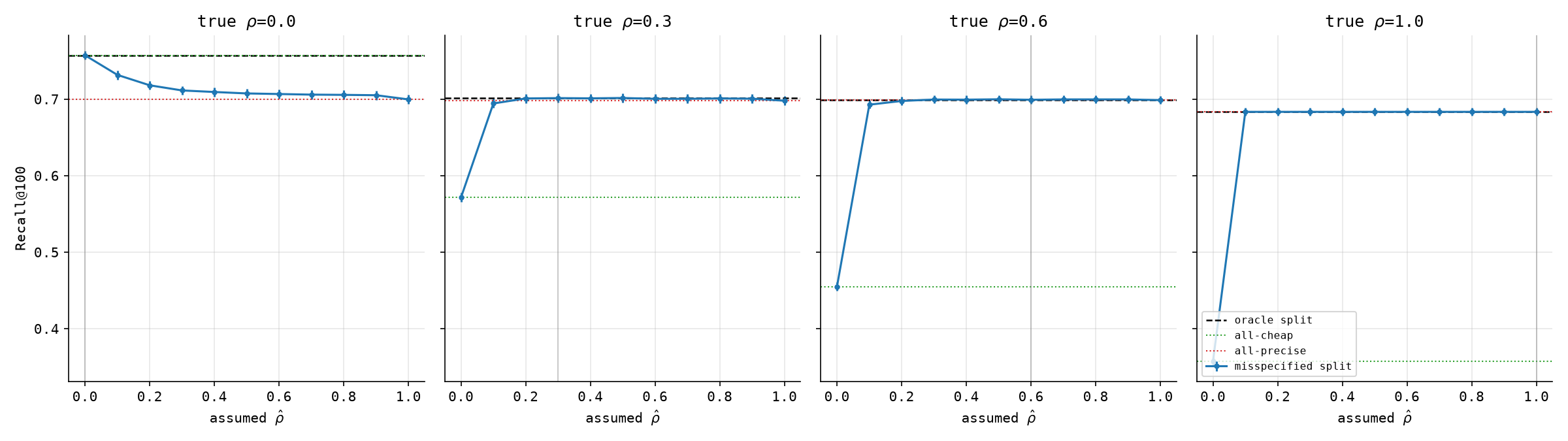
At every true-$\rho$ slice, the misspecified split’s recall is flat and sitting right on the oracle line across almost the whole range of $\hat\rho$, then drops sharply in the last stretch before $\hat\rho=0$. It never falls below both pure baselines — even the worst misspecified point in this experiment stays at or above the weaker of all-cheap and all-precise, so a confidently wrong split is bad, but it does not lose to simply refusing to think about $\rho$ at all here. That is worth stating plainly rather than assuming: “looks principled while it loses,” the worry from the last note, turns out to be bounded by “at least as good as picking a pure strategy at random,” in this setup. Whether that bound holds elsewhere is exactly the kind of claim that needs checking before it gets trusted, not assumed from one figure.

Where This Lands

1. Test misspecification away from the crossing, not at it. The crossing is a point of maximum indifference to allocation by construction; it is the worst place to look for the cost of a wrong belief. I built the experiment there first and got a flat, uninformative result — worth catching before shipping it as “robustness.”
2. The damage is concentrated in one belief, not spread across all wrong beliefs. Any admission that bias might exist — even $\hat\rho=0.1$ — is enough to hedge away nearly all the risk. The catastrophic case is specifically the confident belief that there is none.
3. The two mistakes are not symmetric, and the reason is the same floor argument from the last note. A cheap instrument’s bias floor can coincide with total ignorance (the prior itself); a sharp instrument’s floor cannot. Over-trusting the sharp instrument is a bounded mistake; over-trusting the noisy one, believing it to be unbiased when it is not, is not.

What This Is Not

Still a toy, and this time with a design choice narrowed on purpose. The allocation may be mispriced by $\hat\rho \ne \rho$, but the interpretation of whatever reads get bought uses the true $\rho$ throughout — I am isolating the cost of pricing precision wrong, not compounding it with also misreading your own instruments afterwards. That is a real simplification: in practice you would not know the true $\rho$ for the second step either if you didn’t know it for the first. Folding that back in — a split that is wrong about $\rho$ both when deciding what to buy and when deciding how to weigh what it bought — is the natural next version of this experiment, alongside the misspecified-$\sigma$ question set aside two notes ago. The specific crossover numbers here (one bad column, a sixfold asymmetry, a budget large enough to afford exactly one precise read’s worth) are properties of this simulation at this price and this budget, not constants to carry elsewhere. What I would carry elsewhere is the shape: look for the cost of a wrong prior away from your model’s indifference points, and expect the worst single belief to be the confident absence of the risk you are actually exposed to, not just any wrong number.