The Price of Precision

The budget note ended with a confession I tucked into the footnotes. Every policy in it spent a budget of measurements, and it counted those measurements as if they were all the same price — “treats every engine as equally costly, which no real pipeline does.” I named the lie and walked past it, again. But it is not a footnote. It is the whole reason you have a budget in the first place. You ration measurements because some of them are expensive, and the expensive ones are expensive because they are good. The careful free-energy calculation, the assay, the slow instrument — they cost more precisely because they tell you more.

So the dial I collapsed last time is the one that matters most here. Until now an instrument was a noise level $\sigma$ and nothing else. Now it has a price. A cheap instrument is noisy and costs one unit; a precise instrument is sharp and costs $r$ units, where $r$ is the cost ratio — how many crude reads you forgo to buy one good one. The question is embarrassingly simple to state and I had never asked it: given a fixed budget, should you spend it on a few precise measurements or many crude ones? Precision is not free, and noise is not fatal — you can average it down. So the answer has to turn on a price.

Precision Is a Thing You Buy

Frame it as a race and the shape is already half-visible. The cheap instrument’s error falls as you average: $K$ reads of one compound shrink its noise variance from $\sigma_c^2$ to $\sigma_c^2/K$. The precise instrument starts where the cheap one would need many reads to reach. So for the price of one precise read you could buy $r$ cheap reads instead, and the contest is between the variance those $r$ cheap reads buy you and the variance the single precise read buys you. Somewhere there is a price at which they tie. Below it, precision is a bargain; above it, you are overpaying for sharp numbers you could have approximated by averaging cheap ones.

That tie-point is the entire post. I wanted to know whether it exists, where it sits, and what moves it.

The Setup

I kept the budget note’s machinery so the numbers stay in the same family. Four thousand compounds, hidden qualities $q_i \sim \mathcal{N}(0,1)$, the genuine hits the top $H = 80$. A free initial screen with the cheap instrument scores all of them; I take the top $M = 500$ as a shortlist and spend the budget there. When it is spent I rank the shortlist by posterior mean, take the top $L = 100$, and count how many true hits I recovered. Budget $B = 4000$ throughout; eighty replicates; the bands are one standard error of the mean.

Two instruments observe $q_i$, and each carries the same shared/private split that gave me the correlation knob $\rho$ before — except now the split lives inside one instrument across its own repeated reads:

\[\text{read} = q_i + \underbrace{\sqrt{\rho}\,\sigma\,z_i}_{\text{systematic, shared}} + \underbrace{\sqrt{1-\rho}\,\sigma\,\eta_{ik}}_{\text{private, fresh each read}}.\]

The private part averages away; the systematic part does not. So $K$ reads of one instrument do not floor at zero error — they floor at $\sigma\sqrt{\rho}$, the bias you cannot average out. This is the crucial honesty of the model: the cheap screen and the cheap follow-ups are the same instrument, so they share the cheap instrument’s bias. You cannot launder a systematic error by measuring with the same flawed ruler again.

• all-cheap — spend the whole budget on cheap reads, $\sigma_c = 1.0$, cost $1$, spread uniformly over the shortlist.
• all-precise — spend it all on precise reads, $\sigma_e = 0.35$, cost $r$.
• price-aware split — for each compound, split its share of the budget between the two instruments to minimise posterior variance, the variance-optimal mix at that price.

The posterior is the exact Gaussian update: a standard-normal prior, plus the screen, plus whatever follow-up reads the strategy bought, each weighted by its precision.

The Crossing

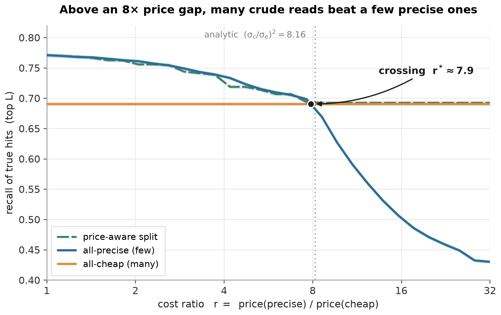
There it is, and it behaves. At $\rho = 0$, when the price gap is small, precision wins clearly — at $r = 1$ the precise reads recover about 0.77 of the hits against the cheap strategy’s 0.69. But the cheap line is flat: its cost never changes, so its recall does not move with $r$. The precise line falls, because every increase in $r$ buys it fewer reads, and around an eight-fold price gap it falls right through the cheap line. Past it, the same budget spent on many crude reads beats a few precise ones — by $r = 32$ the precise strategy has collapsed to 0.43 while the crude one sits unbothered at 0.69. The empirical crossing lands at $r^* \approx 8$.

The price-aware split is the upper envelope, exactly as it should be: it buys precise reads while they are worth it, slides into cheap reads once they are not, and never trails the better pure strategy. It does not reveal a third regime — it just refuses to be on the wrong side of the crossing.

Why Eight

The crossing is not a fitted curiosity; at $\rho = 0$ it has a closed form, and matching the two is the most reassuring thing in the post. One precise read has variance $\sigma_e^2$. To match it by averaging, you need $K$ cheap reads such that $\sigma_c^2 / K = \sigma_e^2$, i.e. $K = (\sigma_c/\sigma_e)^2$. Those $K$ cheap reads cost $K$ units; the one precise read costs $r$. They are an even trade exactly when

\[r^\* = \left(\frac{\sigma_c}{\sigma_e}\right)^2 = \left(\frac{1.0}{0.35}\right)^2 \approx 8.16.\]

The simulation lands a hair under that — the figure’s grey dotted line is the analytic prediction, and the measured crossing sits right on it. Which is the point of computing it at all: the variance algebra and the recall experiment, two different things, agree on the same number. The squaring is the whole story. Precision enters the variance linearly but you pay for it linearly too, so the break-even is set by the square of the noise ratio. A precise instrument that is three times sharper is worth paying up to roughly nine times as much for — and not a unit more.

The Crossing Is Not a Constant

I want to be careful about what $r^* \approx 8$ is and is not, because the tidy closed form invites overreading. The location of the crossing depends on the budget. With more budget, every strategy buys more reads, the cheap strategy’s averaging gets further along its diminishing-returns curve, and the tie-point shifts. The claim that survives is not “the crossing is at eight.” It is weaker and sturdier: a crossing exists, and at $\rho = 0$ it sits at the noise-ratio squared. The number eight is a property of these instruments at this budget. The mechanism — pay for precision only up to the squared noise ratio — is the part I would carry to a different problem.

That distinction is the lesson the last note beat into me. A number the simulation reports is not the same as a number it supports.

The Correlation Returns

It always does. Everything above was at $\rho = 0$ — each read’s bias independent, fully averageable. Turn $\rho$ up, so each instrument’s reads share a systematic bias, and ask where the crossing goes.

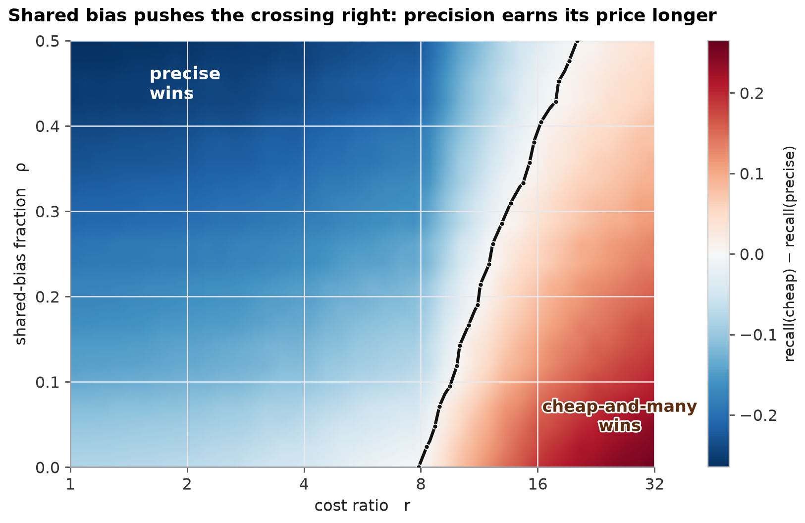
The tie line bends right. The more the cheap reads share a bias, the more overpriced precision has to get before crudeness overtakes it. The reason is the one mechanism this whole sequence keeps circling: averaging defeats noise, never bias. The cheap-and-many strategy lives entirely on averaging — it is only worth anything because $K$ reads beat one. Shared bias is the one error that $K$ does nothing to, and it caps how far the cheap strategy can climb. The precise instrument has a smaller $\sigma$, so its own bias floor $\sigma_e\sqrt{\rho}$ is lower; as $\rho$ rises, the cheap floor $\sigma_c\sqrt{\rho}$ rises faster, and precision keeps its edge over a wider range of prices.

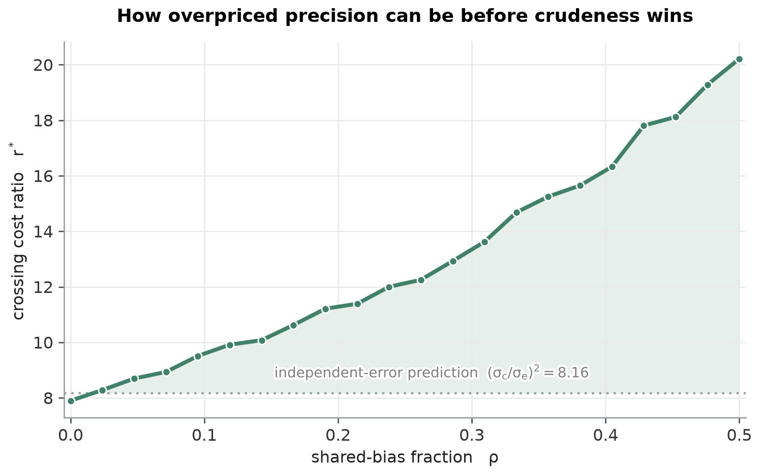
The clean version says it without the heatmap. At $\rho = 0$ the crossing sits on the analytic $(\sigma_c/\sigma_e)^2$; by $\rho = 0.5$ it has climbed past twenty. Shared bias more than doubles the price you should be willing to pay for precision. This is the same thesis the budget note and the disagreement note arrived at from their own directions, now wearing a price tag: independent error is something you can buy your way out of by averaging cheap reads, so when error is independent, cheap-and-many is a real contender and precision is only worth its exact squared premium. Correlated error you cannot average away, so the instrument that has less of it per read is worth a steep markup. The price of precision is set by how much of your noise is the kind averaging can touch.

Where This Lands

The loose thread from the budget note — that not all measurements cost the same — pulls out a crossing and a rule for it:

1. A few precise reads beat many crude ones only below a price gap, and that gap is the squared noise ratio. At $\rho = 0$, pay up to $(\sigma_c/\sigma_e)^2$ for precision and not a unit more. An instrument $k$ times sharper is worth up to $k^2$ times the price.
2. The crossing’s location is a property of the budget; its existence and its $\rho = 0$ value are not. I will defend the mechanism anywhere. I will defend the number eight only for these instruments at this budget.
3. Shared bias raises the price precision is worth, because averaging cannot reach it. Crank $\rho$ to 0.5 and the crossing more than doubles. The cheap-and-many strategy is a bet on averaging, and bias is the bet’s one losing case.

There is a soft spot I built straight into the price-aware split, and naming it is the next thread. The optimal split assumes you know $\sigma_c$, $\sigma_e$, and $\rho$ — it prices precision correctly only because I told it the prices. In the wild you do not know how correlated your instrument’s errors are, and a confident split computed from the wrong $\rho$ is exactly the kind of mistake that looks principled while it loses. That is the misspecified-prior question, and it is where I think this goes next.

---

What This Is Not

A toy, and the same kind of toy as the last three. The instruments are Gaussian noise with a bias term, not docking functions or assays; the budget counts abstract reads, not CPU-hours or reagent cost, and the cost ratio is a clean scalar rather than the messy, regime-dependent thing a real price is. The crossing’s exact value falls out of a posterior I can write in closed form only because I matched the prior to the generating distribution and handed the split the true noise parameters — both luxuries the real world withholds. So $r^* \approx 8$ is a demonstration that a break-even exists and sits where the variance algebra says, not a number to quote for any actual screen. What I would carry out of the simulation is the shape, not the digit: that precision is worth paying for only up to the square of the noise it removes, and that the one thing which raises that ceiling is the share of error your averaging cannot touch.