Pricing Uncertainty Under a Budget

In the last note I wrote down a ranking rule and then walked past it without looking. The memory-enabled pipeline scored each compound by

\[a_i = \bar{s}_i + \lambda\,\sigma_i^{(s)},\]

mean predicted quality plus a bonus for disagreement, and I set $\lambda = 0.5$. I justified the shape of that term at length — a compound the engines argue about should get the benefit of the doubt — but the number I just asserted. Half. Why half? Why not zero, why not two?

That kind of unexamined constant is exactly the thing I accused consensus docking of: a gesture where a measurement should be. So this note is narrow. One question: what is $\lambda$ worth, and what should it be? The answer turned out to depend on something I had not put in the model at all.

The First Answer Is Deflating

Start where the last note left off: every engine scores every compound, then you rank by $\bar{s} + \lambda\sigma$. Sweep $\lambda$ and watch recall.

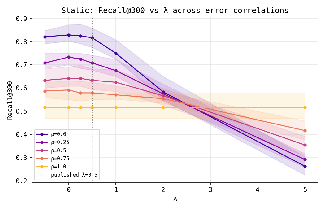
The verdict is almost rude. When observers fail independently ($\rho = 0$), recall is highest at $\lambda = 0$ and slides downward as $\lambda$ grows — at $\lambda = 2$ it has fallen from about 0.83 to 0.58. The disagreement bonus does not help here. It hurts. And the mechanism is obvious in hindsight: a large $\sigma$ is produced just as readily by a worthless compound that one engine wildly overrated as by a genuine hit the engines are split on. Rank by variance and you promote noise. When observers share a bias ($\rho = 1$) the term is simply inert — every engine reports the same value, $\sigma \approx 0$, and $\lambda$ multiplies nothing.

So in the setting of the last note, the honest answer to “why $\lambda = 0.5$?” is: it shouldn’t have been. It should have been roughly zero. When you can measure everything, you do not pay for uncertainty — you average it away and rank by the mean.

I sat with that for a while, because it seemed to demolish the idea. Then I noticed the assumption hiding inside “when you can measure everything.”

You Cannot Measure Everything

The static experiment quietly grants something no real screen ever has: every engine, run on every compound, for free. Real campaigns are not like that. The expensive engines — the careful free-energy calculation, the assay, the experiment — are precisely the ones you cannot afford to run on all six thousand compounds. You run something cheap and fast across the whole library, and then you have a budget: a fixed number of additional, costlier measurements, and a decision about where to spend them.

That decision is where $\lambda$ comes back to life. Spend your next measurement confirming the compound that already looks best (exploit), or investigating the one your estimates are least sure about (explore)? A disagreement bonus is no longer a passive ranking tweak. It is an acquisition rule — it decides what you look at next. This is the exploration–exploitation problem, and stating it that way is itself a sideways step onto a neighboring staircase: the multi-armed bandit people have been climbing for decades.

The rewrite is small but total. Under a Bayesian reading with a standard normal prior, after $n$ measurements of compound $i$ the posterior is

\[\text{mean} = \frac{\sum s_i}{n_i + 1}, \qquad \text{std} = \frac{1}{\sqrt{n_i + 1}},\]

and the rule “measure the compound maximising $\text{mean} + \lambda \cdot \text{std}$” is the classic upper-confidence-bound policy. $\lambda$ is the confidence width — how many standard deviations of optimism you grant the unknown. The exact same symbol, the exact same $\text{mean} + \lambda \cdot \text{std}$, but now it allocates a scarce resource instead of sorting a finished list.

The Setup

I kept everything from the last note that I could, so the numbers stay comparable. Six thousand compounds, hidden qualities $q_i \sim \mathcal{N}(0,1)$, the genuine hits the top $H = 120$. Four engines observe $q_i$ through noise, with the same shared/private split that gives me the correlation knob $\rho$:

\[s_{ik} = q_i + \sigma\left(\sqrt{\rho}\,z_i + \sqrt{1-\rho}\,\eta_{ik}\right).\]

The change is the protocol. One engine scores all six thousand compounds — the cheap initial screen. After that I have a budget of $B$ additional measurements; each one reveals one more engine’s score for one compound of the policy’s choosing. When the budget is spent I rank every compound by its posterior mean and ask the same question as before: of the 120 true hits, how many are in the top $L = 300$? Same metric, same forty replicates, same 16–84 percentile bands.

The policies are the contestants:

• exploit ($\lambda = 0$) — always measure the current highest posterior mean.
• explore — always measure the highest posterior std.
• a family of fixed $\lambda$ — including $\lambda = 0.5$, the value from the last note.
• UCB-adaptive — $\lambda$ grows as $\sqrt{2\ln t}$, the textbook schedule that explores hard early and exploits later.
• Thompson sampling — draw from each posterior and measure the argmax; randomised exploration with no $\lambda$ at all.
• oracle — measure the true top compound every time. Cheating, by construction. It is the ceiling, not a contender.

The Race

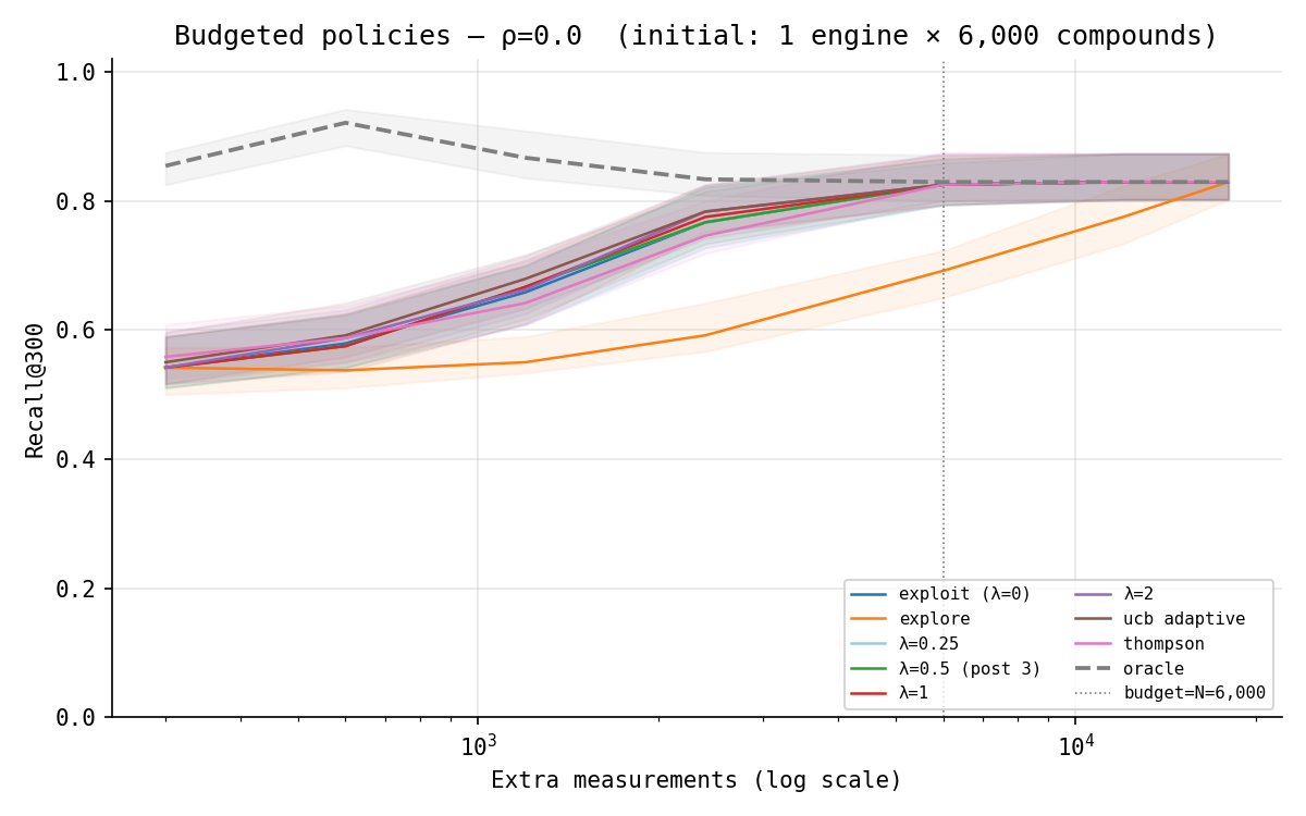
One contrast is large and unambiguous. At a middling budget of 2,400 extra measurements ($\rho = 0$), pure explore is the worst sensible policy by a wide margin — 0.59 — because spending your scarce budget on whatever is most uncertain means pouring measurements into obvious garbage that merely happens to be noisy. The mean-anchored policies all sit far above it, in a tight cluster from about 0.75 to 0.78, against an oracle ceiling of 0.83. That gap — anchor on the mean versus chase pure variance — is the real spread in the figure, and it is the opposite of the static result: there, the $\sigma$ term was a harmless-to-harmful tweak on a finished list; here, ignoring the mean entirely is ruinous, but using $\sigma$ to guide what you resolve next is not.

What is not large is the spread within that cluster. exploit ($\lambda = 0$) and $\lambda = 0.5$ both land at 0.77; $\lambda = 2$ and UCB-adaptive nudge to 0.78; Thompson, whose randomised exploration is the least disciplined of the lot, trails a touch at 0.75. A couple of hits separate them, well inside the bands. It is tempting to read that ordering as “heavier $\lambda$ is better,” and that is exactly the temptation I want to resist, because the gap is the size of noise. Pricing uncertainty clearly went from liability (static) to not-a-liability (budgeted) — the hinge of the note is that a disagreement bonus is the wrong tool for sorting a finished list and a defensible tool for deciding what to measure next. Whether a larger bonus actually beats a smaller one, though, is a claim the figure cannot support on its own — so I went to settle it properly.

I swept $\lambda$ finely at every budget and went looking for the optimum — the value that, if I could name it, would replace the unexamined $0.5$ with an examined one. What I found was not a peak.

I Went Looking For The Right $\lambda$ And Found A Plateau

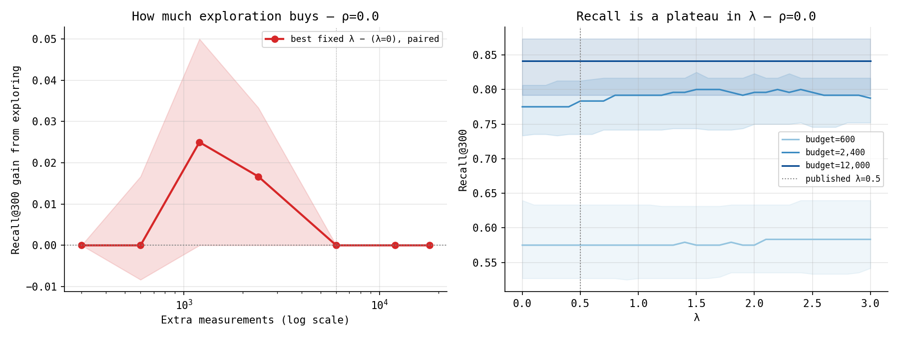
The right panel is the honest picture, and it is humbling. At any fixed budget, recall is nearly flat across the whole range of $\lambda$ — the curves wander inside their own uncertainty bands. There is no sharp best value to find. My first instinct had been to plot “the $\lambda$ that maximises recall” against budget and read off a clean peak; that plot existed, and it swung dramatically up to 2.7 and back down. But it was an artifact. Taking the argmax of a flat, noisy curve manufactures a peak out of nothing — the location of the maximum is just wherever the noise happened to crest. I almost shipped it. It was the same mistake all over again: mistaking a number the data coughed up for a number the data supports.

The left panel is what the question actually deserves. Because every $\lambda$ is evaluated on the same replicates, I can compare them paired — within each run, does the best fixed $\lambda$ beat $\lambda = 0$? — which cancels the run-to-run noise that the flat bands are full of. The gain from exploring, measured honestly:

• At tiny budgets and at large budgets, exactly zero. The extremes are unambiguous.
• In a middle band — a few thousand measurements — a small, real gain: a median of about two to three recovered hits out of 120, positive in roughly four runs out of five, but with a lower band that still grazes zero.

So the shape in budget survives, but shrunken and made honest. Both extremes want $\lambda = 0$, for opposite reasons — too poor to explore (every measurement must buy the likeliest hit; optimism is a luxury) and too rich to need to (with a budget near the library size the problem dissolves back into the static case, where $\lambda = 0$ already won). In between, exploration earns its keep, but only barely, and — this is the part that corrects me — the exact value of $\lambda$ in that band is not determined at all. The recall plateau means $\lambda = 0.5$, $\lambda = 1$, and $\lambda = 2$ are all sitting on the same flat roof. I went in expecting to find that $0.5$ was wrong and the truth was some larger number. What I found is that the truth is a plateau, and $0.5$ is a perfectly ordinary point on it.

This is the real answer to “why half?” Not “it should have been two.” It is: the system is insensitive to $\lambda$ across a wide range, so half was fine — and so was almost anything else. The published value was not under-priced. It was sitting on a flat that I had never checked was flat. The thing that is sharply determined is not the value of $\lambda$ but the two facts bracketing it: that you should anchor on the mean at all rather than chase pure variance, and that the whole exercise only pays inside a middle budget regime. Between those brackets the dial spins freely.

The UCB-adaptive policy is the quiet vindication of this. It never picks a $\lambda$; it lets one decay as the budget burns down, and it tied the best fixed value without being told the budget. On a plateau, not committing to a number is exactly the right move.

The Correlation Returns

There was a second knob in the last note, and it has not gone away. Everything above was at $\rho = 0$, independent observers. What happens when they share a bias?

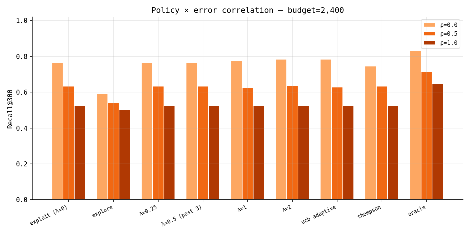
It collapses. At $\rho = 1$ the optimal $\lambda$ is zero at every budget, and the policies flatten into a single undifferentiated bar — exploit, explore, $\lambda = 2$, Thompson, all indistinguishable, all stuck near 0.53. When the engines err together there is no private disagreement to mine; a compound the engines split on is no longer a compound worth a second look, because their split carries no independent information. Exploration has nothing to find, so paying for it buys nothing.

This is the same thesis as the last two notes, arriving from a third direction. The disagreement note: averaging discards information only when observers are independent. The memory note: $V_m$ is largest exactly when observers fail independently. And now: the price you should pay to resolve uncertainty is set by whether that uncertainty is real or shared. Independent error is a signal you can buy your way into. Correlated error only looks like one.

Where This Lands

So the loose thread from the last note pulls out a statement I did not expect, and it is not the one I went looking for. I went in to find the right value of $\lambda$. The lesson is that $\lambda$ was never the sharply determined thing. What is sharp are the brackets around it:

1. Anchor on the mean; never chase pure variance. This is the one large, unambiguous effect in the whole experiment — pure exploration loses by roughly eighteen points of recall. Use disagreement to decide what to resolve next, not as a thing to rank by on its own.
2. The whole exercise only pays inside a middle budget regime. Too broke to explore, too saturated to need to — both extremes want $\lambda = 0$. And inside that middle band the gain is real but small, and the exact $\lambda$ is undetermined: a plateau, not a peak. An adaptive policy that commits to no number does as well as the best fixed one.
3. Independent disagreement is worth resolving; shared bias is not worth a cent. At $\rho = 1$ the entire apparatus flattens. The price of uncertainty is set by whether the uncertainty is real or shared.

The version I shipped last time — a fixed $\lambda = 0.5$, applied to a finished list, with no notion of budget — turns out to have been a fine point on a flat roof, in a corner of the picture where the budget axis was collapsed anyway. It was not wrong. I just never checked whether the dial I had set to 0.5 did anything when I turned it.

That is the part I keep relearning, and this time it nearly bit me twice: once in the original unexamined constant, and once when the data offered me a tidy replacement constant — a $\lambda$ that “peaks at 2.7” — and I almost took it. Both are the same error. The honest move was not to find the right number. It was to discover there was no single right number to find.

---

What This Is Not

Still a toy, and now a slightly larger one. The engines remain Gaussian noise rather than real scoring functions; the “budget” counts abstract measurements, not dollars or CPU-hours, and treats every engine as equally costly, which no real pipeline does. The posterior is exact only because I matched the prior to the generating distribution — a luxury the real world withholds. The recall plateau in $\lambda$, the collapse at $\rho = 1$, the modest middle-budget gain: these are properties of this simulation, demonstrations of a mechanism, not measured constants for any actual screen — and the middle-budget gain in particular is small enough that I would not bet heavily on its size. What survives contact with reality, I think, is the reframing — that the disagreement bonus is an acquisition rule under a budget, not a ranking tweak — and the coarse levers that set its worth: anchor on the mean, spend only in the middle regime, and only when your observers fail independently. Putting real costs and real engines on those axes is, as ever, the harder next step.